Understanding Vector Search and LLMs: From Embeddings to RAG Systems
The advent of embeddings and semantic search has transformed the overall idea of information retrieval. Unlike traditional keyword-based search systems, modern approaches understand the meaning behind words, enabling more intuitive and powerful search capabilities.

If you’re new to the field of Machine Learning and Natural Language Processing, I previously wrote an article on The Evolution of Machine Learning and Natural Language Processing to Transformers which can provide a great starting point.
Embeddings: The Foundation
Embeddings are the mathematical backbone of modern natural language processing and information retrieval systems. They transform words, sentences, or any piece of information into dense numerical vectors in a high-dimensional space (typically 256 to 1024 dimensions). What makes embeddings revolutionary is their ability to capture semantic meaning in these vectors:
Semantic Meaning: Similar concepts end up close to each other in the vector space. For example, “dog” and “puppy” will have similar vector representations.
Compositional Properties: Embeddings can be combined and manipulated mathematically. The classic example is “King — Man + Woman = Queen”, showing how embeddings capture relationships between concepts.
Dimensionality: While words in one-hot encoding would require vectors as large as the vocabulary (millions of dimensions), embeddings compress this information into much smaller, dense vectors.
Contextual Understanding: Modern embedding systems consider the context in which words appear, allowing for nuanced representations where the same word can have different embeddings based on its usage.
Let’s visualize how words get mapped to vectors:
from sentence_transformers import SentenceTransformer
import numpy as np

# Initialize the embedding model
model = SentenceTransformer('all-MiniLM-L6-v2')

# Example sentences
sentences = [
    "The cat sat on the mat",
    "A feline rested on the rug",
    "Dogs are playful pets",
    "The weather is sunny today"
]

# Generate embeddings
embeddings = model.encode(sentences)

# Calculate cosine similarity between first two sentences
def cosine_similarity(v1, v2):
    dot_product = np.dot(v1, v2)
    norm_v1 = np.linalg.norm(v1)
    norm_v2 = np.linalg.norm(v2)
    return dot_product / (norm_v1 * norm_v2)

similarity = cosine_similarity(embeddings[0], embeddings[1])
print(f"Similarity between similar sentences: {similarity:.4f}")
print(f"Embedding dimension: {embeddings.shape[1]}")
Vector Databases and Efficient Search
Vector databases are specialized systems designed to store and query high-dimensional vectors efficiently. They solve several critical challenges:
Scale Challenge: Traditional databases can’t efficiently handle similarity searches in high-dimensional spaces. Vector databases use specialized indexing structures.
Approximate Nearest Neighbor (ANN) Search: Instead of examining every vector (which would be too slow), vector databases use approximation algorithms that trade perfect accuracy for dramatic speed improvements.
Indexing Structures:
- HNSW (Hierarchical Navigable Small World): Creates a layered graph structure for fast navigation
- IVF (Inverted File Index): Partitions vectors into clusters for coarse-to-fine search
- PQ (Product Quantization): Compresses vectors while maintaining search capability
Performance Optimization: Modern vector databases can search millions of vectors in milliseconds using these techniques.
They use sophisticated indexing techniques like:

Cosine Similarity
Cosine similarity is the backbone of vector similarity search. It measures the cosine of the angle between two vectors, providing a similarity score between -1 and 1.
Here’s a visual and mathematical explanation:
import React from 'react';
import { LineChart, Line, XAxis, YAxis, CartesianGrid, ReferenceLine } from 'recharts';

const CosineSimilarityDemo = () => {
  // Generate points for visualization
  const data = [];
  const vector1 = [3, 4];
  const vector2 = [4, 3];

  // Calculate points for vectors
  const points = [
    { x: 0, y: 0 },
    { x: vector1[0], y: vector1[1] },
    { x: 0, y: 0 },
    { x: vector2[0], y: vector2[1] }
  ];

  return (
    <div className="w-full max-w-2xl p-4">
      <div className="mb-4">
        <h3 className="text-lg font-bold mb-2">Cosine Similarity Visualization</h3>
        <LineChart width={400} height={400} margin={{ top: 20, right: 20, bottom: 20, left: 20 }}>
          <CartesianGrid />
          <XAxis type="number" domain={[-1, 5]} />
          <YAxis type="number" domain={[-1, 5]} />
          <ReferenceLine x={0} stroke="#666" />
          <ReferenceLine y={0} stroke="#666" />
          <Line
            data={[points[0], points[1]]}
            type="linear"
            dataKey="y"
            stroke="#8884d8"
            dot={true}
          />
          <Line
            data={[points[2], points[3]]}
            type="linear"
            dataKey="y"
            stroke="#82ca9d"
            dot={true}
          />
        </LineChart>
      </div>
      <div className="text-sm">
        Vector 1 (blue): [3, 4]<br/>
        Vector 2 (green): [4, 3]<br/>
        Cosine Similarity: 0.96
      </div>
    </div>
  );
};

export default CosineSimilarityDemo;
Word2Vec: The Building Blocks
Word2Vec, introduced in 2013, revolutionized how we represent words numerically. Its key innovations include:
Training Paradigms:
- CBOW (Continuous Bag of Words): Predicts a word from its context
- Skip-gram: Predicts context words from a target word
Negative Sampling: Makes training feasible by only updating a small subset of weights
Context Windows: Captures local relationships between words by considering nearby words during training
Emergent Properties: Without explicit programming, Word2Vec learns analogies and relationships between words
Legacy: While newer models have superseded Word2Vec, its principles form the foundation of modern embedding systems
Let’s visualize how it works:

Here’s a practical implementation showing how Word2Vec captures semantic relationships:
from gensim.models import Word2Vec
import numpy as np

# Example training data
sentences = [
    ['king', 'queen', 'palace', 'royal'],
    ['man', 'woman', 'child', 'family'],
    ['computer', 'keyboard', 'mouse', 'screen']
]

# Train Word2Vec model
model = Word2Vec(sentences, vector_size=100, window=2, min_count=1, workers=4)

def analyze_word_relationships(word1, word2, word3):
    """Find word that completes the analogy: word1 is to word2 as word3 is to ???"""
    try:
        result = model.wv.most_similar(
            positive=[word2, word3],
            negative=[word1],
            topn=1
        )
        return result[0]
    except KeyError:
        return None

# Example analogies
analogies = [
    ('man', 'woman', 'king'),  # Expected: queen
    ('computer', 'keyboard', 'phone')  # Expected: touchscreen
]

for w1, w2, w3 in analogies:
    result = analyze_word_relationships(w1, w2, w3)
    if result:
        print(f"{w1} : {w2} :: {w3} : {result[0]} (Score: {result[1]:.2f})")
Modern Language Models (LLMs)
Large Language Models represent the current pinnacle of natural language processing. Large Language Models (LLMs), such as GPT and BERT, use deep learning to understand and generate human-like text. They are trained on massive datasets and fine-tuned for specific tasks like translation, summarization, and semantic search.
Architecture
- Built on the Transformer architecture with self-attention mechanisms
- Multiple layers of neural networks processing information in parallel
- Massive parameter counts (hundreds of billions) enable complex pattern recognition
Capabilities
- Context understanding across long sequences
- Zero-shot and few-shot learning
- Generation of human-like text
- Multi-task ability without specific training
Training Process
- Pre-training on vast amounts of text data
- Fine-tuning for specific tasks
- Instruction tuning for better alignment with human intent
Limitations
High computational requirements, the potential for hallucinations, context window constraints
Let’s break down how modern LLMs work with a comprehensive visualization:

Retrieval-Augmented Generation (RAG)
RAG combines the power of retrieval systems with generative AI. Here’s a complete system architecture:

Let’s implement a basic RAG system:
from sentence_transformers import SentenceTransformer
from typing import List, Dict
import numpy as np
import faiss

class SimpleRAG:
    def __init__(self, embedding_model_name: str = 'all-MiniLM-L6-v2'):
        self.embedding_model = SentenceTransformer(embedding_model_name)
        self.document_store: List[str] = []
        self.index = None

    def add_documents(self, documents: List[str], chunk_size: int = 512):
        """Process and index documents"""
        # Simple chunking strategy
        chunks = []
        for doc in documents:
            # Split into sentences/chunks (simplified)
            doc_chunks = [doc[i:i+chunk_size] for i in range(0, len(doc), chunk_size)]
            chunks.extend(doc_chunks)

        self.document_store = chunks

        # Generate embeddings
        embeddings = self.embedding_model.encode(chunks)

        # Create FAISS index
        dimension = embeddings.shape[1]
        self.index = faiss.IndexFlatL2(dimension)
        self.index.add(np.array(embeddings).astype('float32'))

    def retrieve(self, query: str, k: int = 3) -> List[Dict]:
        """Retrieve relevant documents for a query"""
        # Generate query embedding
        query_embedding = self.embedding_model.encode([query])[0]

        # Search in FAISS
        distances, indices = self.index.search(
            np.array([query_embedding]).astype('float32'), k
        )

        # Return relevant documents with scores
        results = []
        for dist, idx in zip(distances[0], indices[0]):
            results.append({
                'content': self.document_store[idx],
                'score': float(dist)
            })

        return results

    def generate_response(self, query: str, retrieved_docs: List[Dict]) -> str:
        """Generate response using retrieved documents (simplified)"""
        # In a real implementation, this would call an LLM API
        context = "\n".join([doc['content'] for doc in retrieved_docs])
        prompt = f"Context:\n{context}\n\nQuery: {query}\nResponse:"
        return f"Generated response based on {len(retrieved_docs)} retrieved documents"

# Example usage
documents = [
    "RAG systems combine retrieval with generation.",
    "Vector databases store embeddings efficiently.",
    "LLMs process text using attention mechanisms."
]

rag = SimpleRAG()
rag.add_documents(documents)
results = rag.retrieve("How do RAG systems work?")
response = rag.generate_response("How do RAG systems work?", results)
Performance and Scalability
Modern semantic search systems must handle massive scales efficiently:
System Design Considerations:
- Distributed architecture for handling large datasets
- Caching strategies for frequent queries
- Load balancing across multiple servers
- Sharding strategies for vector databases
Optimization Techniques:
- Vector compression through quantization
- Batch processing for efficiency
- Asynchronous updates and lazy loading
- Caching of popular query results
Performance Metrics:
- Query latency (typically milliseconds)
- Throughput (queries per second)
- Recall accuracy vs. speed tradeoffs
- Resource utilization and cost efficiency
Let’s visualize the search performance with different index types:
import React from 'react';
import { BarChart, Bar, XAxis, YAxis, CartesianGrid, Tooltip, Legend } from 'recharts';

const SearchPerformanceComparison = () => {
  const data = [
    {
      name: 'Brute Force',
      '1M Vectors': 1000,
      '10M Vectors': 10000,
      '100M Vectors': 100000,
    },
    {
      name: 'HNSW',
      '1M Vectors': 10,
      '10M Vectors': 15,
      '100M Vectors': 25,
    },
    {
      name: 'IVF',
      '1M Vectors': 20,
      '10M Vectors': 30,
      '100M Vectors': 45,
    },
    {
      name: 'PQ',
      '1M Vectors': 15,
      '10M Vectors': 25,
      '100M Vectors': 40,
    },
  ];

  return (
    <div className="w-full max-w-2xl p-4">
      <h3 className="text-lg font-bold mb-4">Search Latency Comparison (ms)</h3>
      <BarChart width={500} height={300} data={data}>
        <CartesianGrid strokeDasharray="3 3" />
        <XAxis dataKey="name" />
        <YAxis type="log" />
        <Tooltip />
        <Legend />
        <Bar dataKey="1M Vectors" fill="#8884d8" />
        <Bar dataKey="10M Vectors" fill="#82ca9d" />
        <Bar dataKey="100M Vectors" fill="#ffc658" />
      </BarChart>
    </div>
  );
};

export default SearchPerformanceComparison;
Conclusion
The integration of embeddings, vector databases, and large language models has transformed how we interact with and process information. This ecosystem enables:
- Semantic Understanding: Systems now grasp meaning beyond simple keyword matching
- Scalable Solutions: Efficient handling of billions of documents and real-time queries
- Flexible Applications: From search engines to recommendation systems to AI assistants
- Future Potential: Continuing advances in model architecture and hardware enabling new applications
The field continues to evolve rapidly, with improvements in:
- Model efficiency and compression
- Search algorithm optimization
- Integration of multimodal data
- Reduced computational requirements
- Enhanced accuracy and relevance
These technologies together form the backbone of modern AI systems, enabling increasingly sophisticated applications while maintaining practical performance requirements for real-world deployment.